Divide and Conquer
Divide and Conquer
In math and in psychology, ratios are tricky.
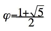
The golden ratio
Source: J. Krueger
In principio erat ratio. ~ St. John, pseudepigraphical
This essay is about a seemingly simple mathematical issue, which, we believe, has far-reaching psychological implications. Before we get into the matter, let us comment on St. John, who opens his gospel by equating the Logos with god. Logos is an Ancient Greek concept of enormous gravity. It can refer to words, phrases, meaning, or communication, but also to the divine order of nature and natural law. One might even see similarities between the Ancient Greek Logos and the Tao of the East. In the modern West, Logos is reduced to The Word, a demotion that began with the Vulgate (Latin) testament, which renders Logos as Verbum. Just imagine, god is a verb. Outside of the bible, the Latins rendered Logos as Ratio, and there we get into the thick of things.
From ratio we get rational and rationality, the gold standard of thinking, the highest reach of psychological functioning.
Another meaning of ratio refers to the result of division, what you get from fractionizing. But how different is this narrow mathematical meaning from the cognitive psychological one? Following Posner (1973), who defined thinking as imagining that which is not immediately given (the stimulus) and considering their relations, Dawes (1988) diagnosed relative, comparative,
and fractionizing thinking as the heart of rationality. Dawes thereby embedded the making of ratios in the achievement of rationality. In the psychology of judgment and decision-making, ratios and their presumed rationality mostly come as part of a greater Bayesian argument. The Reverend Bayes taught how to have a well-behaved mind, a mind that won’t contradict itself.
I remember like it was the day before yesterday, when a classmate in graduate school summarized an article by McCauley and Stitt (1978), which purported to show that social stereotypes are Bayesian, that is, that they are relative. Consider the Japanese. They have – thank god – a low rate of suicide, but this rate may be – and may be perceived to be – a bit larger than in the rest of the world, or in your own country if it is not Japan. Let’s say the perceived prevalence of suicide in Japan is 3%, whereas it is 1% in Luxembourg. According to McCauley & Stitt, this perception differential makes suicide stereotypical of the Japanese and counter-stereotypical of the Luxembourgians and it ought to be expressed as a diagnostic ratio; here 3/1.
McCauley & Stitt argued that the diagnostic ratio is a better and truer measure of stereotyping than the good old-fashioned percentage value obtained for the Japanese. Sure enough, they found that diagnostic ratios are correlated with typicality ratings (‘How typical is committing suicide of the Japanese?’), but in a sustained decade-long quest, my colleagues and I showed that the numerator (% Japanese) does all the work, whereas the denominator (% Luxembourgians) degrades the measure instead of sharpen it (reviewed in Krueger, 2008). Simple percentage estimates for a group are more highly correlated with trait typicality ratings than are diagnostic ratios. We can see this even in McCauley & Stitt’s own data.
Why did McCauley & Stitt think diagnostic ratios are superior? They started from the premise – a prior belief you might say – that all cognition, and hence social cognition, is Bayesian. This means that beliefs can be expressed probabilistically and that a set of beliefs is – or at least should be – consistent in Bayes’ way.
In Bayes’ theorem, the ratio of
the probability that a Japanese person will die by suicide, p(S|J),
divided by the probability that a Luxembourgian will die by suicide,
p(S|L), is equal to the ratio of posterior classification, i.e., the
probability that a suicide is Japanese, p(J|S), over the probability
that a suicide is Luxembourgian, p(L|S), if multiplied by the ratio of
the prior probability that a person is Japanese, p(J), over the prior
probability that a person is Luxembourgian, p(L). In other words, Bayes’
theorem demands the calculation of a ratio of conditional probabilities
so that a person can be classified as Japanese or Luxembourgian given
their differential probabilities of suicide. Elegant as Bayes’ method
is, it is not a good description of how people perceive the typicality
of various traits in social groups
McCauley and others later moved from ratios to difference scores
without much comment. Either way, they probably thought that taking into
account the way a comparison group is being perceived can only improve
measurement and prediction. Yet, ratios and difference scores differ in
important ways. First, ratios are bounded by 0 at the floor, but they
have no ceiling. While 1.0 is the midpoint, lowering the numerator
cannot make the ratio negative, whereas lowering the denominator can
move the ratio towards infinity. This asymmetry yields highly skewed
distributions. In contrast, difference scores make do with a modest and
symmetrical distribution around 0, where the maximum is Xmax – Ymax.
Second – and relatedly – the size of the ratio lets us estimate the
size of the denominator. If the ratio is very large, the denominator is
probably very small. A very large difference score, however, tells us
that both, numerator and denominator are near the endpoints of their
scales, but at opposite ends. At the intuitive-conceptual level, ratios
seem to ‘relativize’ the variable in the numerator, whereas difference
scores seem to ‘correct’ it.
The fascination with ‘relative’ or ‘corrected’ scores runs deep, at least for two reasons. One reason is that Bayes’ theorem provides a standard for rational thought. Rational thought is coherent, and Bayes’ theorem guarantees that the pieces fit together. If one probability is being neglected or ignored altogether, coherent fit can no longer be guaranteed and all mental hell may break loose (Thomas Bayes was a clergyman). The other reason is everyday intuition. This intuition is a funny thing. It says, for example, that ‘more information is always better,’ but then tends to ignore its own advice when making intuitive judgments. Bayesians and other correctors and relativizers tap into the more-is-better intuition when professing abhorrence at the thought that simple heuristic cues may do just fine as decision tools. On their philosophy, rational judgment must divide (or subtract) because failing to do so would leave information on the table – and that would sooner or later result in mayhem.
Relative scores such as ratios or differences are useful if they do better than either of their simple components in predicting a third variable. One reason for why they may not do this is that they are confounded with their components. Difference score are easier to understand than ratios. So let’s start there. Textbooks of statistics teach us that differences are positively correlated with the variable from which we subtract, and they are correlated negatively with the subtracted variable (McNemar, 1969). The correlation, r, is positive between X and X – Y, and it is negative between Y and X – Y.
 Setting aside the variances, or assuming them to be the same for X
and Y, we can see that the numerator is likely to be positive and that
it will be more positive as the correlation between X and Y drops or
becomes negative.
 What, however, can be said about ratios? Will the ratio X/Y be
positively correlated with its numerator X? How can it not be so? As X
increases, then, ceteris paribus, X/Y must increase as well.
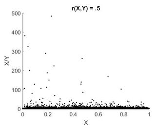
Well, it does not seem at first to work out that way. We ran computer
simulations letting X and Y range over a uniform distribution from 0 to
1. We also varied the correlation between X and Y, but that did not
matter very much. In each simulation most values of X/Y were near 1,
while a few were much larger and even fewer are extremely large. This
result confirms the idea that division yields a highly skewed
distribution. Skew in one
 variable depresses correlations with other variables. For positively correlated values of X and Y (r
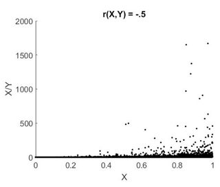
= .5) we find a correlation between X and the ratio X/Y of -.021, and
for a negatively correlated X and Y we find .152. The graphs on the left
show the two scatter plots where X/Y is shown as a function of X. Most
of the ratios are in the lowest section of the scale, while there is a
sprinkling of outliers. When X and Y are positively correlated, the
distribution of X/Y is left-skewed; when the correlation is negative, it
is right-skewed.
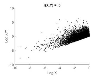
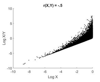
One might be tempted to conclude that a lack of correlation provides proof of independence. Such a conclusion would be hasty because skew may mask true association. A standard correction is to log-transform a skewed variable before correlating it with other variables. When we log-transform the values, we eliminate the inordinate influence of large outlying ones, and a positive association between the numerator, X, and the full ratio, X/Y, emerges.
The second set of two figures shows this. For positively correlated values of X and Y (r = .5) we find a correlation between X and the ratio X/Y of. 514, and for a negatively correlated X and Y we find .831. These correlations are quite large, lending credence to the view that division adds little to what the numerator already accomplishes. Division adds more when the correlation between X and Y becomes increasingly positive. This is interesting because it means that ‘relativizing’ a variable X by dividing it by variable Y is most informative inasmuch as the differences between them (between a sampled value of X and a sampled value of Y) become smaller.
 The skew of the ratio distribution has another problematic
consequence. We know that the arithmetic mean is likely to be higher
than the conceptual central point of 1.0, which we would get when X = Y.
Since it is possible to get a ratio of X/Y > 2 but impossible to get
one < 0, most sample means will be > 1. In a symmetrical
distribution, the mean is an unbiased estimate of the true average
(i.e., the mean of an infinitely large sample); it is neither
systematically too small nor too large, and it does not systematically
vary as a function of the sample size. This is not so in a skewed
distribution. In a skewed distribution, the mean will
 creep up as sample size N increases because larger samples make it
more likely that very rare but very large values (here, ratios) will be
captured. If they are captured, they pull up the mean. Since we know
that a ratio can drift towards infinity as the denominator gets
infinitesimally small, we also know that a very very large sample will
very very probably yield a mean that is virtually, practically, or
morally infinite. We would not want that to happen because the result
would be uninterpretable.
To illustrate the rise of the mean as a function of N, we performed a series
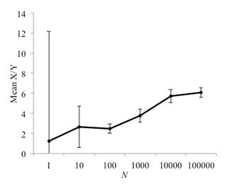 of simulations. The final figure shows the sample means of X/Y
computed over 1,000 simulations for each of the 7 samples sizes along a
logarithmic scale. Note that the mean ratio goes up, as does the
precision with which it is estimated (the bars around each mean express
the standard error, which is the standard deviation of the sampled means
divided by the square root of their number).
There is no reason to abandon all hope and all ratios. But in many psychological contexts it is good practice to ask if as much has been gained as was hoped. One would not want to rationalize the use of ratios after the fact. We recommend reporting ratios along with their ingredient variables so that one can appreciate the absolute levels from which the ratios arose. And of course, some ratios are beautiful, such as the golden one in the picture at the top. Closing the circle - if you allow a geometrical metaphor- Fra Luca Pacioli, the great renaissance mathematician, observed that “Like God, the Divine Proportion is always similar to itself.”
The fascination with ‘relative’ or ‘corrected’ scores runs deep, at least for two reasons. One reason is that Bayes’ theorem provides a standard for rational thought. Rational thought is coherent, and Bayes’ theorem guarantees that the pieces fit together. If one probability is being neglected or ignored altogether, coherent fit can no longer be guaranteed and all mental hell may break loose (Thomas Bayes was a clergyman). The other reason is everyday intuition. This intuition is a funny thing. It says, for example, that ‘more information is always better,’ but then tends to ignore its own advice when making intuitive judgments. Bayesians and other correctors and relativizers tap into the more-is-better intuition when professing abhorrence at the thought that simple heuristic cues may do just fine as decision tools. On their philosophy, rational judgment must divide (or subtract) because failing to do so would leave information on the table – and that would sooner or later result in mayhem.
Relative scores such as ratios or differences are useful if they do better than either of their simple components in predicting a third variable. One reason for why they may not do this is that they are confounded with their components. Difference score are easier to understand than ratios. So let’s start there. Textbooks of statistics teach us that differences are positively correlated with the variable from which we subtract, and they are correlated negatively with the subtracted variable (McNemar, 1969). The correlation, r, is positive between X and X – Y, and it is negative between Y and X – Y.

Source: J. Krueger

Ratios plotted against their numerator
Source: P. Heck

Positive (right) skew when X and Y are negatively correlated.
Source: P. Heck
One might be tempted to conclude that a lack of correlation provides proof of independence. Such a conclusion would be hasty because skew may mask true association. A standard correction is to log-transform a skewed variable before correlating it with other variables. When we log-transform the values, we eliminate the inordinate influence of large outlying ones, and a positive association between the numerator, X, and the full ratio, X/Y, emerges.
The second set of two figures shows this. For positively correlated values of X and Y (r = .5) we find a correlation between X and the ratio X/Y of. 514, and for a negatively correlated X and Y we find .831. These correlations are quite large, lending credence to the view that division adds little to what the numerator already accomplishes. Division adds more when the correlation between X and Y becomes increasingly positive. This is interesting because it means that ‘relativizing’ a variable X by dividing it by variable Y is most informative inasmuch as the differences between them (between a sampled value of X and a sampled value of Y) become smaller.

Linear relationship emerging after log transformation
Source: P. Heck

Strong linear association between X and X/Y.
Source: P. Heck
To illustrate the rise of the mean as a function of N, we performed a series

The biasing effect of sample size on expected mean ratio.
Source: P. Heck
There is no reason to abandon all hope and all ratios. But in many psychological contexts it is good practice to ask if as much has been gained as was hoped. One would not want to rationalize the use of ratios after the fact. We recommend reporting ratios along with their ingredient variables so that one can appreciate the absolute levels from which the ratios arose. And of course, some ratios are beautiful, such as the golden one in the picture at the top. Closing the circle - if you allow a geometrical metaphor- Fra Luca Pacioli, the great renaissance mathematician, observed that “Like God, the Divine Proportion is always similar to itself.”

